New Study Shows Prediction Target and Loss Choice Dramatically Shape Diffusion Model Quality
Grafy Research Lab’s paper reveals how loss‑space weighting and architectural bottlenecks interact with prediction targets in diffusion models.
 Source: Grafy Research Lab
Diffusion models can be trained to predict clean data (), noise (), or velocity (), and the loss can be measured in any of these three spaces. A new paper from the Grafy Research Lab shows that the nine possible prediction‑loss pairings are not interchangeable in practice, especially when the network contains a low‑rank bottleneck.
What design choices does the paper examine?
The authors consider all nine combinations of prediction target { , , } and loss space { , , }. While the three quantities are linked by simple affine transforms, finite‑capacity networks do not achieve the ideal algebraic equivalence. The study isolates two independent factors: (1) the prediction space – which quantity the network outputs – and (2) the loss space – where the squared‑error is computed. By varying each factor separately, the authors can attribute performance differences to either choice.
How does loss‑space selection relate to timestep weighting?
For a fixed prediction target, changing the loss space is mathematically equivalent to applying a deterministic reweighting of timesteps during training. Proposition 1 in the paper proves that the loss computed in a space different from the prediction target can be expressed as the original loss multiplied by a factor that depends only on the noise level . In other words, using an ‑loss while predicting is the same as training with an ‑loss but giving higher importance to certain timesteps.
The authors provide a heuristic analysis (Proposition 2) that predicts when this reweighting helps. If a model is more sensitive to early (high‑noise) timesteps, an ‑loss can improve sample quality; conversely, when low‑noise timesteps dominate learning, an ‑loss may be preferable. This insight explains why recent diffusion works such as Min‑SNR or P2 weighting, which explicitly reshape the timestep distribution, often report gains.
Why do architectural bottlenecks affect prediction targets differently?
A central contribution is the analysis of a rank‑ linear bottleneck that compresses the ‑dimensional noisy input . Theorem 4 shows that for noise () and velocity () prediction, the bottleneck imposes an irreducible squared‑error floor of . By contrast, clean‑data prediction () can exploit low‑dimensional structure of natural images, allowing it to bypass the limit.
The paper also derives error‑amplification factors when converting a prediction back to a clean‑data estimate. For noise prediction the conversion scales the error by , and for velocity prediction by (Proposition 6). Combining these scalings with the bottleneck floor yields distinct necessary conditions on for each prediction target (Corollary 7). In practice this means that a highly compressed model may still generate good images if it predicts , but will struggle if it predicts or .
What empirical evidence supports the theory?
The authors validate their claims on three datasets – CIFAR‑10, Imagenette, and ImageNet‑256 – using both a conventional U‑Net and the JiT transformer introduced by Li and He (2026). Experiments without a bottleneck confirm the loss‑space reweighting effect: models trained with ‑loss outperform ‑loss when the timestep schedule emphasizes early steps.
When a bottleneck is introduced, the predicted errors follow the theoretical floor. Figure 3 shows samples generated by JiT‑B/8 on Imagenette under three prediction choices. The ‑prediction column produces recognizable images, the ‑prediction column is heavily degraded, and the ‑prediction column collapses to pure noise, despite all three sharing the same 130 M‑parameter architecture and 100 Heun steps. This visual evidence aligns with the derived error bounds: noise‑prediction errors match the floor, while clean‑data prediction benefits from data manifold structure.
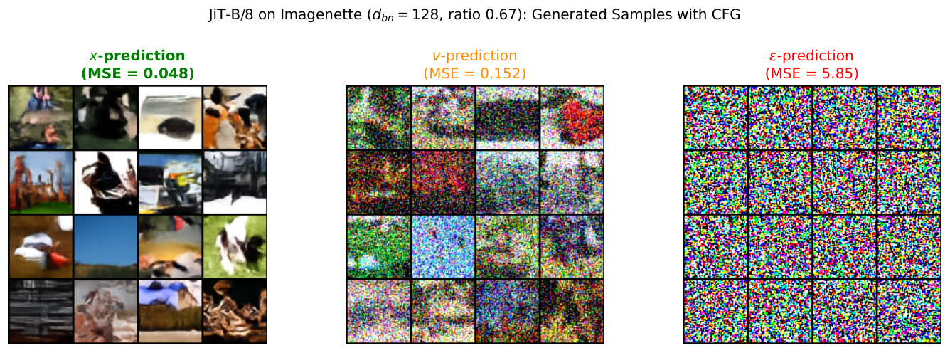
The bottleneck‑width sweep further reveals that increasing reduces the gap for and predictions, but the improvement plateaus once exceeds the intrinsic data dimension, confirming the low‑dimensional advantage of ‑prediction.
How can creators and developers use these insights with Grafy?
Grafy’s Reader app lets you upload the PDF of the paper and query the model for specific sections, making it easy to explore the proofs of Proposition 1 or Theorem 4 without leaving the workspace. If you are prototyping a diffusion model, the Code studio can be used to implement the loss‑space reweighting described in the paper – simply replace a standard ‑loss with an ‑loss and multiply by the timestep‑dependent factor provided in the appendix. For quick experimentation, the Chat interface can run small‑scale diffusion training loops on cloud models (OpenRouter, Vertex AI, etc.) and let you compare , , and predictions under different bottleneck ranks.
By integrating the paper’s theoretical guidance, developers can decide whether to allocate more capacity to the encoder (to raise ) or to switch prediction targets, depending on their hardware budget and desired sample quality. The combination of Reader, Code, and Chat offers a low‑friction workflow to test these trade‑offs on your own datasets.
Frequently asked questions
Does changing the loss space always improve generation quality?
Not necessarily. The paper shows that loss‑space changes are equivalent to timestep reweighting, which can help if the model benefits from emphasizing certain timesteps. When the schedule already favours low‑noise steps, an ‑loss may be optimal, and switching to ‑loss could hurt quality.
Can a strong bottleneck be compensated by predicting clean data ()?
Yes. Theoretical analysis (Theorem 4) and experiments indicate that ‑prediction can exploit low‑dimensional data structure and avoid the error floor that limits and predictions. However, this advantage diminishes if the data manifold is high‑dimensional or the bottleneck rank is very small.
How can I test the paper’s predictions on my own diffusion model?
Upload the model’s training script to Grafy Code, add the loss‑weighting factor from Proposition 1, and run a short training run with different bottleneck ranks. Use Grafy Reader to reference the paper’s equations while you code, and query Grafy Chat for debugging tips. Comparing FID scores across the nine prediction‑loss combos will let you verify the reported trends.
More news

Local Agent Harnesses Scale From 0.75B to 4.7B, New Study Finds Mingbird Leads
A Grafy Research Lab paper maps five locally‑run agent harnesses across four open‑weight models, showing the Mingbird harness outperforms others at every size.

CARE Introduces Retrieval‑Aligned Semantic IDs for Generative Retrieval
Grafy Research Lab unveils CARE, a new SID tokenizer that quantizes in a retrieval‑aligned space.
Study Shows Reusing Old Vector Index Only Delays, Not Eliminates, Re‑encoding
A new Grafy Research Lab paper finds that reusing an existing embedding index merely postpones full re‑encoding.